Geometría básica

En este artículo consideraremos las operaciones básicas sobre puntos en el espacio euclidiano, que constituyen el fundamento de toda la geometría analítica. Para cada punto $\mathbf r$ consideraremos el vector $\vec{\mathbf r}$ dirigido de $\mathbf 0$ a $\mathbf r$. Más adelante no distinguiremos entre $\mathbf r$ y $\vec{\mathbf r}$ y usaremos el término punto como sinónimo de vector.

Operaciones lineales

Tanto los puntos 2D como los 3D forman un espacio lineal, lo que significa que para ellos están definidas la suma de puntos y la multiplicación de un punto por un número. Aquí están esas implementaciones básicas para 2D:

struct point2d {
    ftype x, y;
    point2d() {}
    point2d(ftype x, ftype y): x(x), y(y) {}
    point2d& operator+=(const point2d &t) {
        x += t.x;
        y += t.y;
        return *this;
    }
    point2d& operator-=(const point2d &t) {
        x -= t.x;
        y -= t.y;
        return *this;
    }
    point2d& operator*=(ftype t) {
        x *= t;
        y *= t;
        return *this;
    }
    point2d& operator/=(ftype t) {
        x /= t;
        y /= t;
        return *this;
    }
    point2d operator+(const point2d &t) const {
        return point2d(*this) += t;
    }
    point2d operator-(const point2d &t) const {
        return point2d(*this) -= t;
    }
    point2d operator*(ftype t) const {
        return point2d(*this) *= t;
    }
    point2d operator/(ftype t) const {
        return point2d(*this) /= t;
    }
};
point2d operator*(ftype a, point2d b) {
    return b * a;
}

Y los puntos 3D:

struct point3d {
    ftype x, y, z;
    point3d() {}
    point3d(ftype x, ftype y, ftype z): x(x), y(y), z(z) {}
    point3d& operator+=(const point3d &t) {
        x += t.x;
        y += t.y;
        z += t.z;
        return *this;
    }
    point3d& operator-=(const point3d &t) {
        x -= t.x;
        y -= t.y;
        z -= t.z;
        return *this;
    }
    point3d& operator*=(ftype t) {
        x *= t;
        y *= t;
        z *= t;
        return *this;
    }
    point3d& operator/=(ftype t) {
        x /= t;
        y /= t;
        z /= t;
        return *this;
    }
    point3d operator+(const point3d &t) const {
        return point3d(*this) += t;
    }
    point3d operator-(const point3d &t) const {
        return point3d(*this) -= t;
    }
    point3d operator*(ftype t) const {
        return point3d(*this) *= t;
    }
    point3d operator/(ftype t) const {
        return point3d(*this) /= t;
    }
};
point3d operator*(ftype a, point3d b) {
    return b * a;
}

Aquí ftype es algún tipo usado para las coordenadas, habitualmente int, double o long long.

Producto punto

Definición

El producto punto (o escalar) $\mathbf a \cdot \mathbf b$ de los vectores $\mathbf a$ y $\mathbf b$ se puede definir de dos maneras equivalentes. Geométricamente es el producto de la longitud del primer vector por la longitud de la proyección del segundo vector sobre el primero. Como se puede ver en la imagen de abajo, esta proyección no es otra cosa que $|\mathbf a| \cos \theta$, donde $\theta$ es el ángulo entre $\mathbf a$ y $\mathbf b$. Así, $\mathbf a\cdot \mathbf b = |\mathbf a| \cos \theta \cdot |\mathbf b|$.

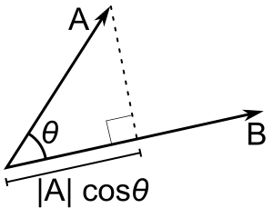
El producto punto tiene algunas propiedades notables:

1. $\mathbf a \cdot \mathbf b = \mathbf b \cdot \mathbf a$
2. $(\alpha \cdot \mathbf a)\cdot \mathbf b = \alpha \cdot (\mathbf a \cdot \mathbf b)$
3. $(\mathbf a + \mathbf b)\cdot \mathbf c = \mathbf a \cdot \mathbf c + \mathbf b \cdot \mathbf c$

Es decir, es una función conmutativa que es lineal respecto de ambos argumentos. Denotemos los vectores unitarios como

$$\mathbf e_x =$$$$\begin{pmatrix} 1 \ 0 \ 0 \end{pmatrix}$$, \mathbf e_y = $$\begin{pmatrix} 0 \ 1 \ 0 \end{pmatrix}$$, \mathbf e_z = $$\begin{pmatrix} 0 \ 0 \ 1 \end{pmatrix}$$.

Con esta notación podemos escribir el vector $\mathbf r = (x;y;z)$ como $r = x \cdot \mathbf e_x + y \cdot \mathbf e_y + z \cdot \mathbf e_z$. Y como para los vectores unitarios

$$\mathbf e_x\cdot \mathbf e_x = \mathbf e_y\cdot \mathbf e_y = \mathbf e_z\cdot \mathbf e_z = 1,\ \mathbf e_x\cdot \mathbf e_y = \mathbf e_y\cdot \mathbf e_z = \mathbf e_z\cdot \mathbf e_x = 0$$

vemos que, en términos de coordenadas, para $\mathbf a = (x_1;y_1;z_1)$ y $\mathbf b = (x_2;y_2;z_2)$ se cumple

$$\mathbf a\cdot \mathbf b = (x_1 \cdot \mathbf e_x + y_1 \cdot\mathbf e_y + z_1 \cdot\mathbf e_z)\cdot( x_2 \cdot\mathbf e_x + y_2 \cdot\mathbf e_y + z_2 \cdot\mathbf e_z) = x_1 x_2 + y_1 y_2 + z_1 z_2$$

Esa es también la definición algebraica del producto punto. A partir de esto podemos escribir funciones que lo calculen.

ftype dot(point2d a, point2d b) {
    return a.x * b.x + a.y * b.y;
}
ftype dot(point3d a, point3d b) {
    return a.x * b.x + a.y * b.y + a.z * b.z;
}

Al resolver problemas se debe usar la definición algebraica para calcular productos punto, pero conviene tener presente la definición geométrica y las propiedades para aplicarlas.

Propiedades

Podemos definir muchas propiedades geométricas mediante el producto punto. Por ejemplo

1. Norma de $\mathbf a$ (longitud al cuadrado): $|\mathbf a|^2 = \mathbf a\cdot \mathbf a$
2. Longitud de $\mathbf a$: $|\mathbf a| = \sqrt{\mathbf a\cdot \mathbf a}$
3. Proyección de $\mathbf a$ sobre $\mathbf b$: $\dfrac{\mathbf a\cdot\mathbf b}{|\mathbf b|}$
4. Ángulo entre vectores: $\arccos \left(\dfrac{\mathbf a\cdot \mathbf b}{|\mathbf a| \cdot |\mathbf b|}\right)$
5. Del punto anterior se ve que el producto punto es positivo si el ángulo entre ellos es agudo, negativo si es obtuso e igual a cero si son ortogonales, es decir, si forman un ángulo recto.

Nótese que todas estas funciones no dependen del número de dimensiones, de modo que serán las mismas en el caso 2D y en el 3D:

ftype norm(point2d a) {
    return dot(a, a);
}
double abs(point2d a) {
    return sqrt(norm(a));
}
double proj(point2d a, point2d b) {
    return dot(a, b) / abs(b);
}
double angle(point2d a, point2d b) {
    return acos(dot(a, b) / abs(a) / abs(b));
}

Para ver la siguiente propiedad importante debemos mirar el conjunto de puntos $\mathbf r$ para los cuales $\mathbf r\cdot \mathbf a = C$ para alguna constante fija $C$. Se puede ver que este conjunto de puntos es exactamente el conjunto de puntos para los cuales la proyección sobre $\mathbf a$ es el punto $C \cdot \dfrac{\mathbf a}{|\mathbf a| ^ 2}$ y forman un hiperplano ortogonal a $\mathbf a$. En la figura de abajo se puede ver el vector $\mathbf a$ junto con varios de esos vectores que tienen el mismo producto punto con él, en 2D:

En 2D estos vectores formarán una recta; en 3D formarán un plano. Nótese que este resultado nos permite definir una recta en 2D como $\mathbf r\cdot \mathbf n=C$ o $(\mathbf r - \mathbf r_0)\cdot \mathbf n=0$, donde $\mathbf n$ es un vector ortogonal a la recta, $\mathbf r_0$ es cualquier vector que ya esté sobre la recta y $C = \mathbf r_0\cdot \mathbf n$. De la misma manera se puede definir un plano en 3D.

Producto cruz

Definición

Supongamos que tenemos tres vectores $\mathbf a$, $\mathbf b$ y $\mathbf c$ en el espacio 3D unidos en un paralelepípedo como en la imagen de abajo:

¿Cómo calcularíamos su volumen? De la escuela sabemos que hay que multiplicar el área de la base por la altura, que es la proyección de $\mathbf a$ sobre la dirección ortogonal a la base. Eso significa que si definimos $\mathbf b \times \mathbf c$ como el vector ortogonal tanto a $\mathbf b$ como a $\mathbf c$ y cuya longitud es igual al área del paralelogramo formado por $\mathbf b$ y $\mathbf c$, entonces $|\mathbf a\cdot (\mathbf b\times\mathbf c)|$ será igual al volumen del paralelepípedo. Por consistencia diremos que $\mathbf b\times \mathbf c$ estará siempre dirigido de modo que la rotación del vector $\mathbf b$ hacia el vector $\mathbf c$, vista desde el punto de $\mathbf b\times \mathbf c$, sea siempre antihoraria (véase la imagen de abajo).

Esto define el producto cruz (o vectorial) $\mathbf b\times \mathbf c$ de los vectores $\mathbf b$ y $\mathbf c$ y el producto mixto $\mathbf a\cdot(\mathbf b\times \mathbf c)$ de los vectores $\mathbf a$, $\mathbf b$ y $\mathbf c$.

Algunas propiedades notables de los productos cruz y mixto:

1. $\mathbf a\times \mathbf b = -\mathbf b\times \mathbf a$

2. $(\alpha \cdot \mathbf a)\times \mathbf b = \alpha \cdot (\mathbf a\times \mathbf b)$

3. Para cualquier $\mathbf b$ y $\mathbf c$ existe exactamente un vector $\mathbf r$ tal que $\mathbf a\cdot (\mathbf b\times \mathbf c) = \mathbf a\cdot\mathbf r$ para cualquier vector $\mathbf a$.
   En efecto, si hubiera dos de esos vectores $\mathbf r_1$ y $\mathbf r_2$ entonces $\mathbf a\cdot (\mathbf r_1 - \mathbf r_2)=0$ para todos los vectores $\mathbf a$, lo cual solo es posible cuando $\mathbf r_1 = \mathbf r_2$.

4. $\mathbf a\cdot (\mathbf b\times \mathbf c) = \mathbf b\cdot (\mathbf c\times \mathbf a) = -\mathbf a\cdot( \mathbf c\times \mathbf b)$

5. $(\mathbf a + \mathbf b)\times \mathbf c = \mathbf a\times \mathbf c + \mathbf b\times \mathbf c$. En efecto, para todos los vectores $\mathbf r$ se cumple la cadena de igualdades:

   $$\mathbf r\cdot( (\mathbf a + \mathbf b)\times \mathbf c) = (\mathbf a + \mathbf b) \cdot (\mathbf c\times \mathbf r) = \mathbf a \cdot(\mathbf c\times \mathbf r) + \mathbf b\cdot(\mathbf c\times \mathbf r) = \mathbf r\cdot (\mathbf a\times \mathbf c) + \mathbf r\cdot(\mathbf b\times \mathbf c) = \mathbf r\cdot(\mathbf a\times \mathbf c + \mathbf b\times \mathbf c)$$

   Lo que demuestra $(\mathbf a + \mathbf b)\times \mathbf c = \mathbf a\times \mathbf c + \mathbf b\times \mathbf c$ por el punto 3.

6. $|\mathbf a\times \mathbf b|=|\mathbf a| \cdot |\mathbf b| \sin \theta$ donde $\theta$ es el ángulo entre $\mathbf a$ y $\mathbf b$, ya que $|\mathbf a\times \mathbf b|$ es igual al área del paralelogramo formado por $\mathbf a$ y $\mathbf b$.

Dado todo esto y que para los vectores unitarios se cumple la siguiente ecuación

$$\mathbf e_x\times \mathbf e_x = \mathbf e_y\times \mathbf e_y = \mathbf e_z\times \mathbf e_z = \mathbf 0,\ \mathbf e_x\times \mathbf e_y = \mathbf e_z,\mathbf e_y\times \mathbf e_z = \mathbf e_x,\mathbf e_z\times \mathbf e_x = \mathbf e_y$$

podemos calcular el producto cruz de $\mathbf a = (x_1;y_1;z_1)$ y $\mathbf b = (x_2;y_2;z_2)$ en forma coordenada:

$$\mathbf a\times \mathbf b = (x_1 \cdot \mathbf e_x + y_1 \cdot \mathbf e_y + z_1 \cdot \mathbf e_z)\times (x_2 \cdot \mathbf e_x + y_2 \cdot \mathbf e_y + z_2 \cdot \mathbf e_z) =$$

$$(y_1 z_2 - z_1 y_2)\mathbf e_x + (z_1 x_2 - x_1 z_2)\mathbf e_y + (x_1 y_2 - y_1 x_2)\mathbf e_z$$

Lo cual también se puede escribir de forma más elegante:

$$\mathbf a\times \mathbf b =$$$$\begin{vmatrix}\mathbf e_x & \mathbf e_y & \mathbf e_z \ x_1 & y_1 & z_1 \ x_2 & y_2 & z_2 \end{vmatrix}$$,~a\cdot(b\times c) = $$\begin{vmatrix} x_1 & y_1 & z_1 \ x_2 & y_2 & z_2 \ x_3 & y_3 & z_3 \end{vmatrix}$$

Aquí $| \cdot |$ denota el determinante de una matriz.

Alguna forma de producto cruz (concretamente el producto seudoescalar) también se puede implementar en el caso 2D. Si quisiéramos calcular el área del paralelogramo formado por los vectores $\mathbf a$ y $\mathbf b$ computaríamos $|\mathbf e_z\cdot(\mathbf a\times \mathbf b)| = |x_1 y_2 - y_1 x_2|$. Otra forma de obtener el mismo resultado es multiplicar $|\mathbf a|$ (base del paralelogramo) por la altura, que es la proyección del vector $\mathbf b$ sobre el vector $\mathbf a$ rotado $90^\circ$, que a su vez es $\widehat{\mathbf a}=(-y_1;x_1)$. Es decir, calcular $|\widehat{\mathbf a}\cdot\mathbf b|=|x_1y_2 - y_1 x_2|$.

Si tenemos en cuenta el signo, el área será positiva si la rotación de $\mathbf a$ a $\mathbf b$ (es decir, desde el punto de vista de $\mathbf e_z$) se realiza en sentido antihorario y negativa en caso contrario. Eso define el producto seudoescalar. Nótese que también es igual a $|\mathbf a| \cdot |\mathbf b| \sin \theta$, donde $\theta$ es el ángulo de $\mathbf a$ a $\mathbf b$ contado en sentido antihorario (y negativo si la rotación es horaria).

¡Implementemos todo esto!

point3d cross(point3d a, point3d b) {
    return point3d(a.y * b.z - a.z * b.y,
                   a.z * b.x - a.x * b.z,
                   a.x * b.y - a.y * b.x);
}
ftype triple(point3d a, point3d b, point3d c) {
    return dot(a, cross(b, c));
}
ftype cross(point2d a, point2d b) {
    return a.x * b.y - a.y * b.x;
}

Propiedades

En cuanto al producto cruz, es igual al vector cero si y solo si los vectores $\mathbf a$ y $\mathbf b$ son colineales (forman una recta común, es decir, son paralelos). Lo mismo vale para el producto mixto: es igual a cero si y solo si los vectores $\mathbf a$, $\mathbf b$ y $\mathbf c$ son coplanares (forman un plano común).

De esto podemos obtener ecuaciones universales que definen rectas y planos. Una recta se puede definir mediante su vector director $\mathbf d$ y un punto inicial $\mathbf r_0$, o por dos puntos $\mathbf a$ y $\mathbf b$. Se define como $(\mathbf r - \mathbf r_0)\times\mathbf d=0$ o como $(\mathbf r - \mathbf a)\times (\mathbf b - \mathbf a) = 0$. En cuanto a los planos, se pueden definir por tres puntos $\mathbf a$, $\mathbf b$ y $\mathbf c$ como $(\mathbf r - \mathbf a)\cdot((\mathbf b - \mathbf a)\times (\mathbf c - \mathbf a))=0$ o por un punto inicial $\mathbf r_0$ y dos vectores directores que yacen en ese plano $\mathbf d_1$ y $\mathbf d_2$: $(\mathbf r - \mathbf r_0)\cdot(\mathbf d_1\times \mathbf d_2)=0$.

En 2D el producto seudoescalar también puede usarse para comprobar la orientación entre dos vectores, porque es positivo si la rotación del primero al segundo es antihoraria y negativo en caso contrario. Y, por supuesto, puede usarse para calcular áreas de polígonos, lo cual se describe en otro artículo. El producto mixto puede usarse para el mismo propósito en el espacio 3D.

Ejercicios

Intersección de rectas

Hay muchas formas posibles de definir una recta en 2D y no hay que dudar en combinarlas. Por ejemplo, tenemos dos rectas y queremos encontrar sus puntos de intersección. Podemos decir que todos los puntos de la primera recta se pueden parametrizar como $\mathbf r = \mathbf a_1 + t \cdot \mathbf d_1$, donde $\mathbf a_1$ es el punto inicial, $\mathbf d_1$ es la dirección y $t$ es algún parámetro real. En cuanto a la segunda recta, todos sus puntos deben satisfacer $(\mathbf r - \mathbf a_2)\times \mathbf d_2=0$. De esto podemos hallar fácilmente el parámetro $t$:

$$(\mathbf a_1 + t \cdot \mathbf d_1 - \mathbf a_2)\times \mathbf d_2=0 \quad\Rightarrow\quad t = \dfrac{(\mathbf a_2 - \mathbf a_1)\times\mathbf d_2}{\mathbf d_1\times \mathbf d_2}$$

Implementemos una función para intersectar dos rectas.

point2d intersect(point2d a1, point2d d1, point2d a2, point2d d2) {
    return a1 + cross(a2 - a1, d2) / cross(d1, d2) * d1;
}

Intersección de planos

Sin embargo, a veces puede ser difícil usar intuiciones geométricas. Por ejemplo, se dan tres planos definidos por puntos iniciales $\mathbf a_i$ y direcciones $\mathbf d_i$ y se quiere encontrar su punto de intersección. Se puede notar que basta con resolver el sistema de ecuaciones:

$$\{\begin{array}{l}\mathbf{r}\cdot {\mathbf{n}}_1={\mathbf{a}}_1\cdot {\mathbf{n}}_1,\\ \mathbf{r}\cdot {\mathbf{n}}_2={\mathbf{a}}_2\cdot {\mathbf{n}}_2,\\ \mathbf{r}\cdot {\mathbf{n}}_3={\mathbf{a}}_3\cdot {\mathbf{n}}_3\end{array}$$$$\begin{cases}\mathbf r\cdot \mathbf n_1 = \mathbf a_1\cdot \mathbf n_1, \ \mathbf r\cdot \mathbf n_2 = \mathbf a_2\cdot \mathbf n_2, \ \mathbf r\cdot \mathbf n_3 = \mathbf a_3\cdot \mathbf n_3\end{cases}$$

En lugar de pensar en un enfoque geométrico, se puede elaborar uno algebraico que se obtiene de inmediato. Por ejemplo, dado que ya implementaste una clase de punto, te será fácil resolver este sistema usando la regla de Cramer, porque el producto mixto es simplemente el determinante de la matriz obtenida a partir de los vectores como columnas:

point3d intersect(point3d a1, point3d n1, point3d a2, point3d n2, point3d a3, point3d n3) {
    point3d x(n1.x, n2.x, n3.x);
    point3d y(n1.y, n2.y, n3.y);
    point3d z(n1.z, n2.z, n3.z); 
    point3d d(dot(a1, n1), dot(a2, n2), dot(a3, n3));
    return point3d(triple(d, y, z),
                   triple(x, d, z),
                   triple(x, y, d)) / triple(n1, n2, n3);
}

Ahora puedes intentar encontrar por tu cuenta enfoques para las operaciones geométricas habituales, para acostumbrarte a todo esto.